How to Read Frequency Analysis of Audio File

Understanding Audio data, Fourier Transform, FFT and Spectrogram features for a Speech Recognition Arrangement

An introduction to audio data analysis (sound analysis) using python

Overview

A huge amount of audio data is being generated every 24-hour interval in almost every organisation. Audio data yields substantial strategic insights when it is easily attainable to the information scientists for fuelling AI engines and analytics. Organizations that have already realized the power and importance of the information coming from the sound data are leveraging the AI (Artificial Intelligence) transcribed conversations to improve their staff grooming, client services and enhancing overall customer experience.

On the other manus, there ar e organizations that are non able to put their audio data to better employ because of the following barriers — i. They are not capturing information technology. ii. The quality of the data is bad. These barriers tin limit the potential of Auto Learning solutions (AI engines) they are going to implement. Information technology is really important to capture all possible data and likewise in good quality.

This article provides a stride-wise guide to outset with audio data processing. Though this volition assist y'all get started with basic assay, It is never a bad idea to become a basic understanding of the audio waves and basic signal processing techniques before jumping into this field. Yous tin can click here and check out my article on audio waves. That article provides a bones understanding of sound waves and also explains a fleck about dissimilar audio codecs.

Before going farther, let'due south listing out the content we are going to comprehend in this article. Allow's go through each of the post-obit topics sequentially—

1. Reading Audio Files
2. Fourier Transform (FT)
3. Fast Fourier Transform (FFT)
4. Spectrogram
5. Speech communication Recognition using Spectrogram Features
6. Decision

1. Reading Sound Files

LIBROSA

LibROSA is a python library that has most every utility y'all are going to demand while working on sound information. This rich library comes upwards with a large number of different functionalities. Here is a quick light on the features —

1. Loading and displaying characteristics of an audio file.
2. Spectral representations
3. Characteristic extraction and Manipulation
4. Time-Frequency conversions
5. Temporal Partitioning
6. Sequential Modeling…etc

Equally this library is huge, we are not going to talk about all the features information technology carries. We are merely going to use a few mutual features for our understanding.

Here is how y'all can install this library existent quick —

                              pypi                : pip install librosa
                conda                : conda install -c conda-forge librosa            

Loading Sound into Python

Librosa supports lots of sound codecs. Although .wav(lossless) is widely used when sound information analysis is concerned. Once you have successfully installed and imported libROSA in your jupyter notebook. You tin can read a given sound file by simply passing the file_path to librosa.load() function.

librosa.load() —> part returns 2 things — 1. An array of amplitudes. 2. Sampling rate. The sampling rate refers to 'sampling frequency' used while recording the audio file. If you keep the argument sr = None , it volition load your audio file in its original sampling rate. (Annotation: You can specify your custom sampling charge per unit every bit per your requirement, libROSA tin can upsample or downsample the signal for you). Look at the following image —

sampling_rate = 16k says that this sound was recorded(sampled) with a sampling frequency of 16k. In other words, while recording this file we were capturing 16000 amplitudes every second. Thus, If we want to know the duration of the audio, we can simply divide the number of samples (amplitudes) by the sampling-rate every bit shown below —

"Yes you can play the audio inside your jupyter-notebook."

IPython gives us a widget to play audio files through notebook.

Visualizing Audio

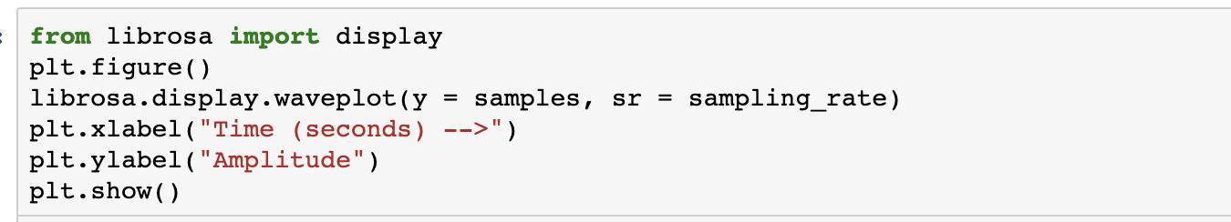
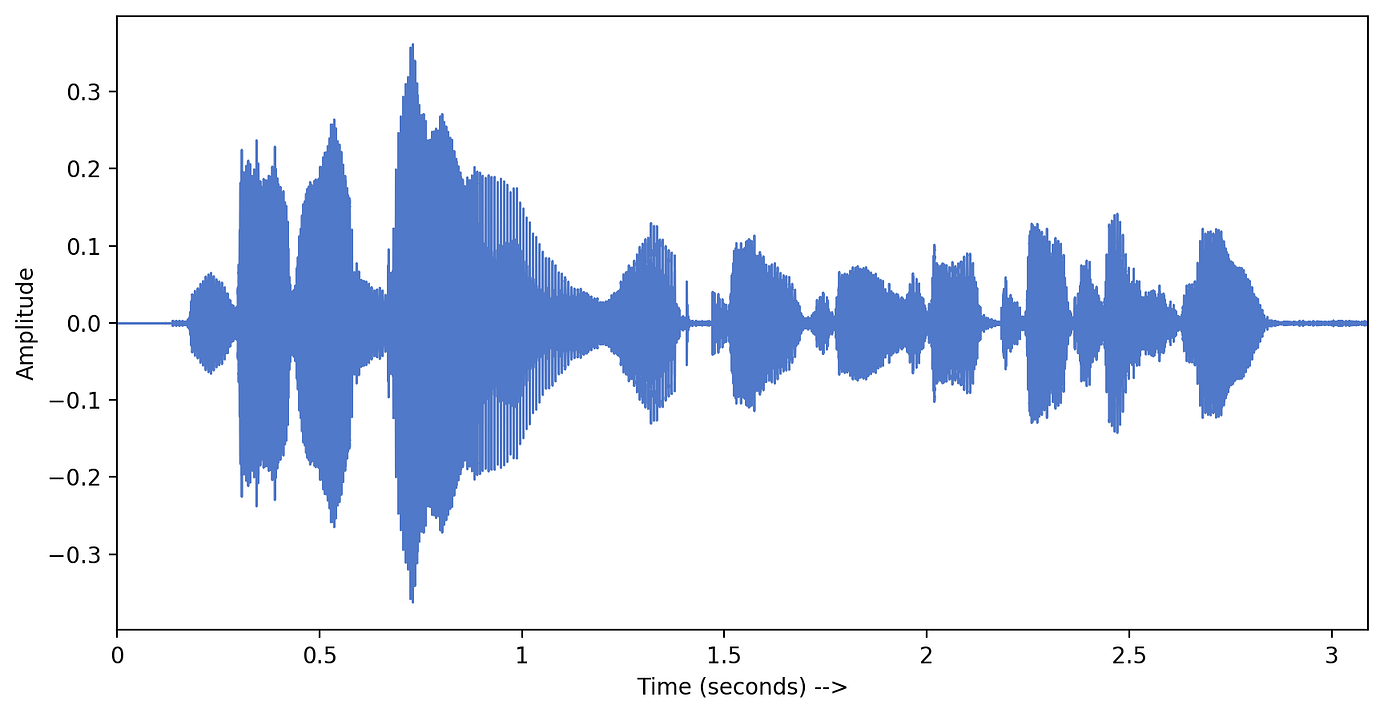
We have got amplitudes and sampling-rate from librosa. We can easily plot these amplitudes with time. LibROSA provides a utility function waveplot() equally shown below —

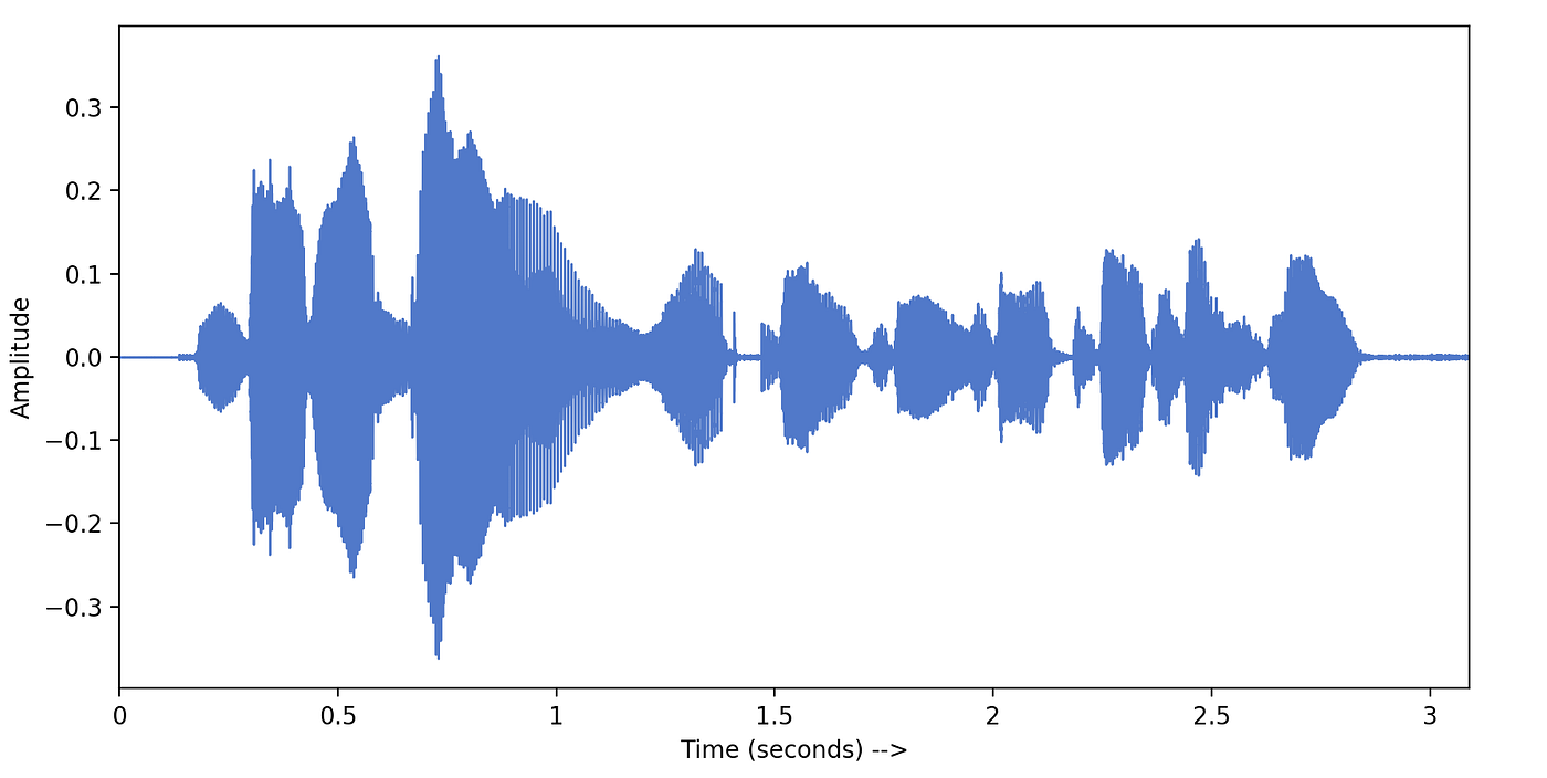
This visualization is chosen the time-domain representation of a given signal. This shows us the loudness (amplitude) of sound wave irresolute with time. Here amplitude = 0 represents silence. (From the definition of sound waves — This aamplitude is actually the amplitude of air particles which are aquiver because of the pressure change in the temper due to sound).

These amplitudes are non very informative, as they only talk well-nigh the loudness of audio recording. To amend empathize the audio signal, it is necessary to transform it into the frequency-domain. The frequency-domain representation of a signal tells us what different frequencies are nowadays in the point. Fourier Transform is a mathematical concept that can catechumen a continuous signal from fourth dimension-domain to frequency-domain. Permit's larn more than about Fourier Transform.

two. Fourier Transform (FT)

An audio bespeak is a complex signal composed of multiple 'single-frequency sound waves' which travel together every bit a disturbance(pressure-change) in the medium. When sound is recorded we just capture the resultant amplitudes of those multiple waves. Fourier Transform is a mathematical concept that tin decompose a signal into its constituent frequencies . Fourier transform does not just requite the frequencies present in the betoken, It also gives the magnitude of each frequency present in the signal.

Inverse Fourier Transform is just the opposite of the Fourier Transform. It takes the frequency-domain representation of a given signal as input and does mathematically synthesize the original indicate.

Let's run across how we can utilise Fourier transformation to convert our sound signal into its frequency components —

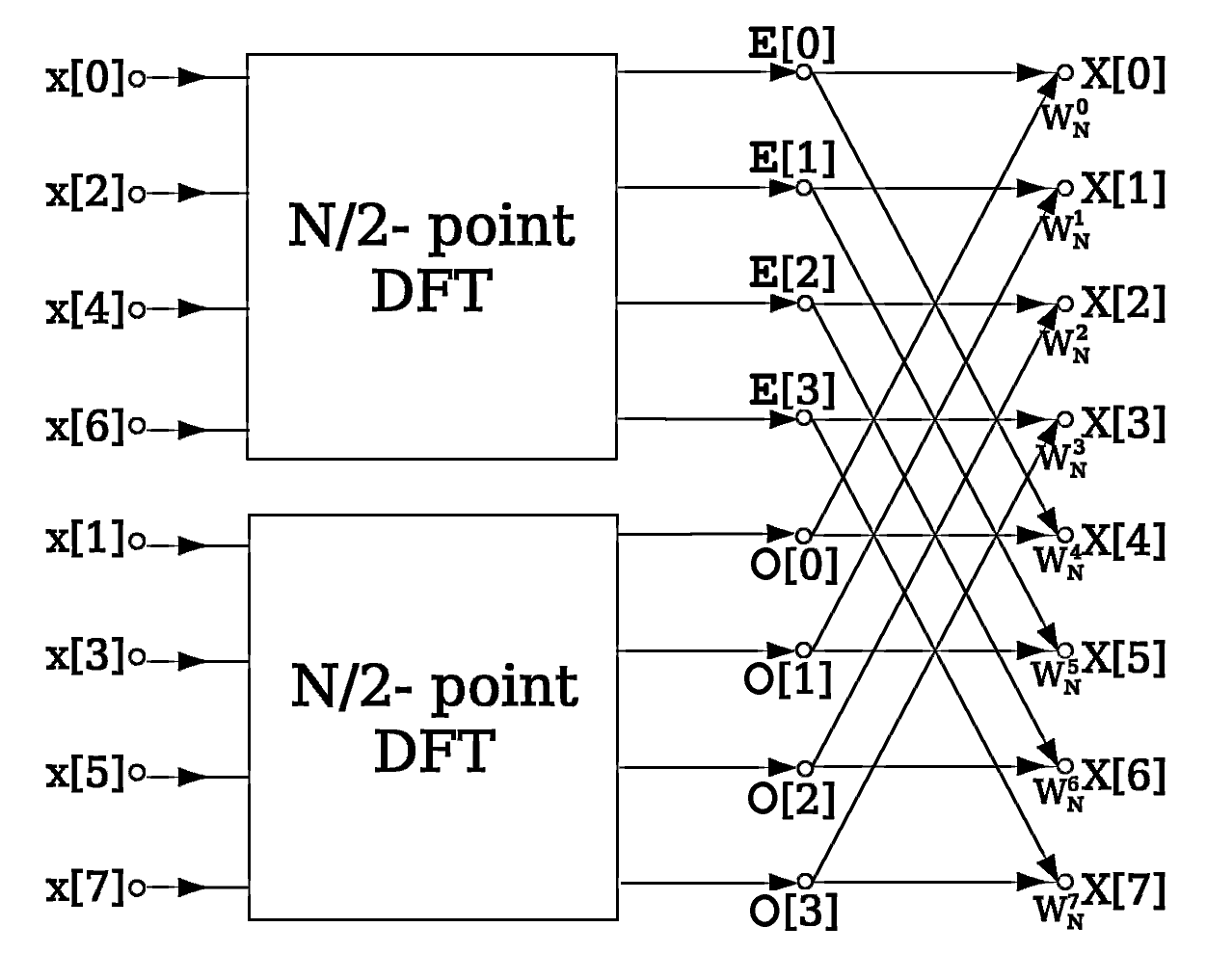
iii. Fast Fourier Transform (FFT)

Fast Fourier Transformation(FFT) is a mathematical algorithm that calculates Discrete Fourier Transform(DFT) of a given sequence. The only divergence between FT(Fourier Transform) and FFT is that FT considers a continuous signal while FFT takes a discrete signal as input. DFT converts a sequence (discrete signal) into its frequency constituents only like FT does for a continuous signal. In our instance, we accept a sequence of amplitudes that were sampled from a continuous audio point. DFT or FFT algorithm can convert this time-domain discrete signal into a frequency-domain.

FFT algorithm overview

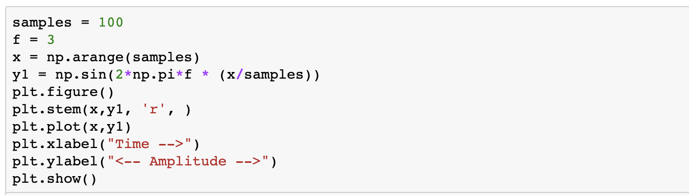
Simple Sine Wave to Sympathize FFT

To understand the output of FFT, permit's create a simple sine wave. The following slice of code creates a sine wave with a sampling rate = 100, amplitude = 1 and frequency = three . Amplitude values are calculated every 1/100th 2d (sampling rate) and stored into a list chosen y1. We will pass these detached amplitude values to calculate DFT of this bespeak using the FFT algorithm.

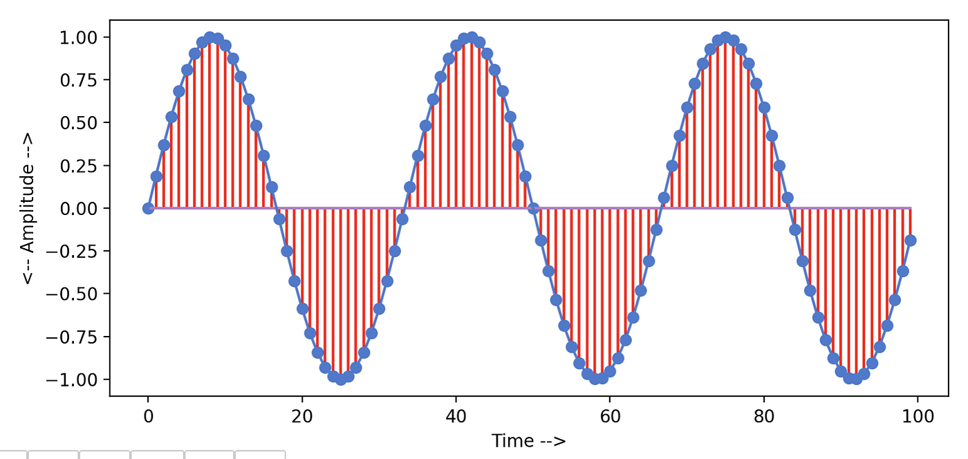
If y'all plot these discrete values(y1) keeping sample number on x-axis and aamplitude value on y-centrality, it generates a nice sine wave plot as the following screenshot shows —

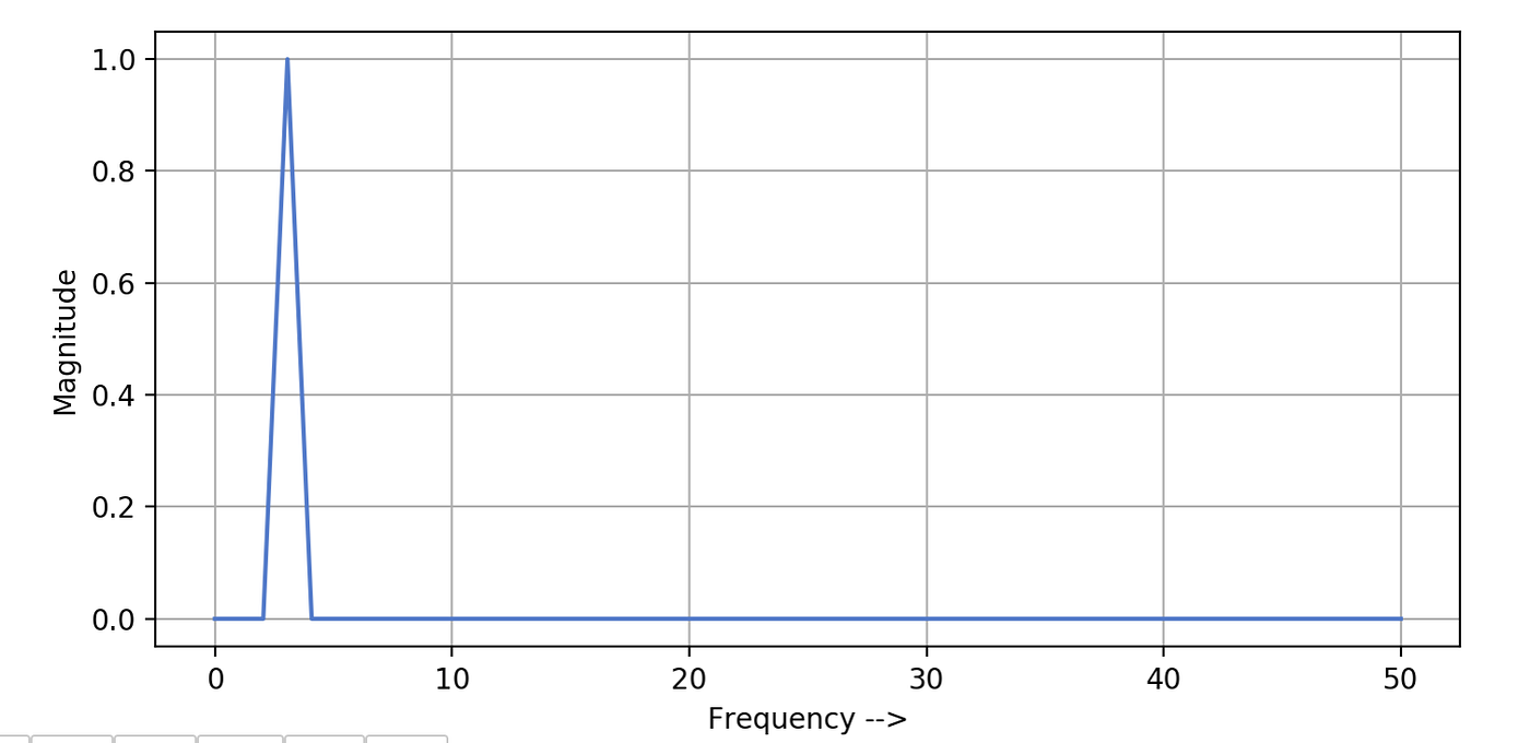
Now we accept a sequence of amplitudes stored in listing y1. Nosotros will pass this sequence to the FFT algorithm implemented past scipy. This algorithm returns a list yf of complex-valued amplitudes of the frequencies constitute in the bespeak. The get-go one-half of this list returns positive-frequency-terms, and the other half returns negative-frequency-terms which are like to the positive ones. You can pick out whatever ane half and calculate absolute values to represent the frequencies present in the signal. Following function takes samples equally input and plots the frequency graph —

In the following graph, we have plotted the frequencies for our sine wave using the above fft_plot function. You can see this plot clearly shows the single frequency value present in our sine wave, which is 3. Also, information technology shows amplitude related to this frequency which we kept ane for our sine wave.

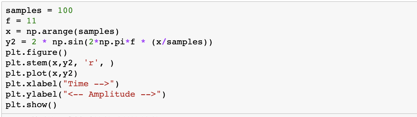
To bank check out the output of FFT for a signal having more one frequency, Permit'southward create another sine moving ridge. This time we will keep sampling rate = 100, aamplitude = 2 and frequency value = 11 . Following code generates this indicate and plots the sine moving ridge —

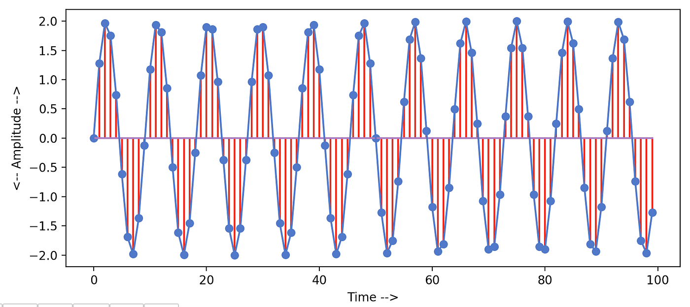
Generated sine moving ridge looks similar the below graph. Information technology would have been smoother if we had increased the sampling rate. Nosotros have kept the sampling rate = 100 because after nosotros are going to add this signal to our old sine wave.

Manifestly FFT office will show a single spike with frequency = eleven for this wave also. But nosotros want to see what happens if we add these two signals of the same sampling rate but the different frequency and aamplitude values. Here sequence y3 will represent the resultant point.

If nosotros plot the signal y3, information technology looks something similar this —

If we pass this sequence (y3) to our fft_plot function. Information technology generates the following frequency graph for u.s.. It shows two spikes for the ii frequencies nowadays in our resultant signal. So the presence of one frequency does not bear on the other frequency in the signal. Also, ane thing to observe is that the magnitudes of the frequencies are in line with our generated sine waves.

FFT on our Sound signal

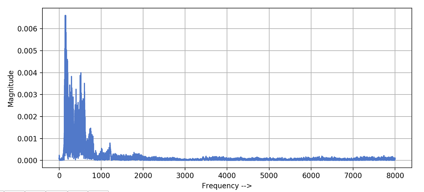
Now that we take seen how this FFT algorithm gives us all the frequencies in a given signal. let's try to pass our original audio betoken into this function. Nosotros are using the same audio prune nosotros loaded earlier into the python with a sampling rate = 16000.

Now, wait at the following frequency plot. This '3-2nd long' indicate is composed of thousands of different frequencies. Magnitudes of frequency values > 2000 are very small equally about of these frequencies are probably due to the noise. We are plotting frequencies ranging from 0 to 8kHz because our signal was sampled at 16k sampling rate and according to the Nyquist sampling theorem, information technology should simply posses frequencies ≤ 8000Hz (16000/two).

Strong frequencies are ranging from 0 to 1kHz simply considering this audio prune was human voice communication. We know that in a typical human speech this range of frequencies dominates.

We got frequencies Merely where is the Fourth dimension data?

4. Spectrogram

why spectrogram

Suppose you lot are working on a Voice communication Recognition task. You have an sound file in which someone is speaking a phrase (for example: How are y'all). Your recognition organisation should be able to predict these iii words in the same order (1. 'how', ii. 'are', iii. 'you'). If you remember, in the previous practise we broke our point into its frequency values which volition serve equally features for our recognition system. Just when nosotros applied FFT to our signal, it gave us only frequency values and we lost the track of fourth dimension information. Now our system won't be able to tell what was spoken first if we employ these frequencies as features. We need to find a dissimilar style to calculate features for our system such that it has frequency values along with the time at which they were observed. Here Spectrograms come up into the motion picture.

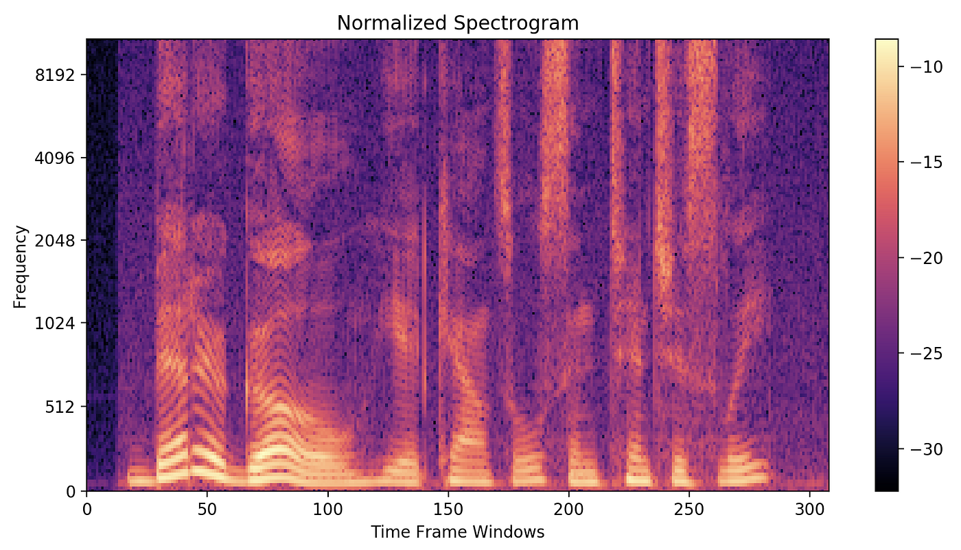
Visual representation of frequencies of a given signal with time is called Spectrogram. In a spectrogram representation plot — one axis represents the time, the second centrality represents frequencies and the colors stand for magnitude (amplitude) of the observed frequency at a item time. The following screenshot represents the spectrogram of the same sound point we discussed earlier. Bright colors correspond potent frequencies. Similar to before FFT plot, smaller frequencies ranging from (0–1kHz) are strong(vivid).

Creating and Plotting the spectrogram

Idea is to break the audio signal into smaller frames(windows) and calculate DFT (or FFT) for each window. This mode nosotros will be getting frequencies for each window and window number volition represent the time. Every bit window i comes kickoff, window 2 next…and and so on. It'southward a good exercise to proceed these windows overlapping otherwise we might lose a few frequencies. Window size depends upon the problem you are solving.

For a typical speech communication recognition task, a window of xx to 30ms long is recommended. A man can't possibly speak more than one phoneme in this time window. So keeping the window this much smaller we won't lose whatever phoneme while classifying. The frame (window) overlap can vary from 25% to 75% as per your need, generally, it is kept 50% for spoken language recognition.

In our spectrogram adding, nosotros will proceed the window duration 20ms and an overlap of 50% among the windows. Because our signal is sampled at 16k frequency, each window is going to accept (16000 * xx * 0.001) = 320 amplitudes. For an overlap of fifty%, we need to go forward by (320/2) = 160 amplitude values to get to the adjacent window. Thus our stride value is 160.

Have a wait at the spectrogram function in the following image. In line-18 we are making a weighting window( Hanning ) and multiplying it with amplitudes earlier passing it to FFT part in line-twenty. Weighting window is used here to handle discontinuity of this small signal(minor point from a single frame) before passing it to the DFT algorithm. To learn more virtually why the weighting window is necessary — click hither.

A python function to calculate spectrogram features —

The output of the FFT algorithm is a list of complex numbers (size = window_size /2) which represent amplitudes of different frequencies inside the window. For our window of size 320, we volition get a list of 160 amplitudes of frequency bins which represent frequencies from 0 Hz — 8kHz (as our sampling rate is 16k) in our example.

Going forrad, Absolute values of those complex-valued amplitudes are calculated and normalized. The resulting second matrix is your spectrogram. In this matrix rows and columns represent window frame number and frequency bin while values represent the strength of the frequencies.

5. Spoken communication Recognition using Spectrogram Features

We know how to generate a spectrogram now, which is a 2d matrix representing the frequency magnitudes along with time for a given signal. At present call up of this spectrogram as an image. You take converted your sound file into the following image.

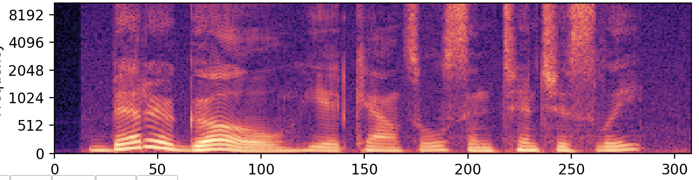
This reduces information technology to an image classification problem . This prototype represents your spoken phrase from left to right in a timely manner. Or consider this as an prototype where your phrase is written from left to right, and all you need to practice is identify those hidden English characters.

Given a parallel corpus of English language text, nosotros can train a deep learning model and build a speech recognition system of our own. Here are two well known open up-source datasets to try out —

              Popular open source datasets —
i. LibriSpeech ASR corpus
2. Common Voice Massively-Multilingual Speech Corpus            

Popular choices of deep learning architectures can be understood from the post-obit dainty research papers —

1. Wave2Lettter (Facebook Research)
2. Deep Speech, Deep Oral communication 2 and Deep Speech 3(Baidu Inquiry)
3. Listen, Nourish and Spell (Google Brain)
4. JASPER (NVIDIA)

half-dozen. Conclusion

This article shows how to bargain with audio data and a few audio analysis techniques from scratch. Besides, it gives a starting point for edifice speech recognition systems. Although, Above research shows very promising results for the recognition systems, yet many don't come across speech communication recognition as a solved problem considering of the following pitfalls —

1. Speech recognition models presented by the researchers are really big (circuitous), which makes them hard to train and deploy.
2. These systems don't work well when multiple people are talking.
3. These systems don't work well when the quality of the audio is bad.
4. They are really sensitive to the accent of the speaker thus requires training for every different emphasis.

There are huge opportunities in this field of enquiry. Improvements can be done from the information training signal of view (past creating meliorate features) and too from the model architecture point of view (by presenting a more than robust and scalable deep learning architecture).

Originally published hither.

Cite this commodity: Google Scholar Link

Thanks for reading, please let me know your comments/feedback.

How to Read Frequency Analysis of Audio File

Source: https://towardsdatascience.com/understanding-audio-data-fourier-transform-fft-spectrogram-and-speech-recognition-a4072d228520

Share this post